Saying Goodbye to Geometric Networks

When many of us started receiving deprecation warnings for geometric networks from ESRI years ago, we shook our heads ruefully. Who has time to migrate? Not now! If you are like me, you have kicked the can down the road year after year, and now 2026 is here. As of March 1st, geometric networks are no longer officially supported, and we haven't migrated yet. If you are in the same boat, do not worry. In this blog series, we will take you step by step through our UN migration at the City of Grants Pass. You will share our suffering, learn from our mistakes, and by the end I hope you will feel new confidence for tackling this migration in your municipality. So let's begin!

Meet Grants Pass

Grants Pass is a small city of 40,000 people, nestled in the Rogue Valley of Southern Oregon, just north of the Oregon Caves. Geographically bound by steep hillslopes, our city is small enough to have only a single staff member (me) assigned to utilities, but large enough that we encounter many of the data quality issues that plague larger cities.

Not only am I solely responsible for migrating sewer, storm and water networks from geometric to utility networks, but I have to do this as a side project while adding new development and maintaining our existing data. I suspect you have more in common with me than you would like... the good news is that this is totally doable, as a side project, without pissing off your boss.

Why Wastewater?

We begin our migration with the wastewater network, because this is the simplest network among the three. Our stormwater network is intertwined with assets from the Grants Pass Irrigation District, necessitating custom attribute rules, and the water distribution network involves the largest collection of device types and assemblies, increasing the complexity of the import mapping. By tackling wastewater first, we can learn to walk before we run, and familiarize ourselves with the basic import workflow. After we have conquered these challenges, and produced a working wastewater utility network, the additional complexities of storm and water distribution will seem much more tractable.

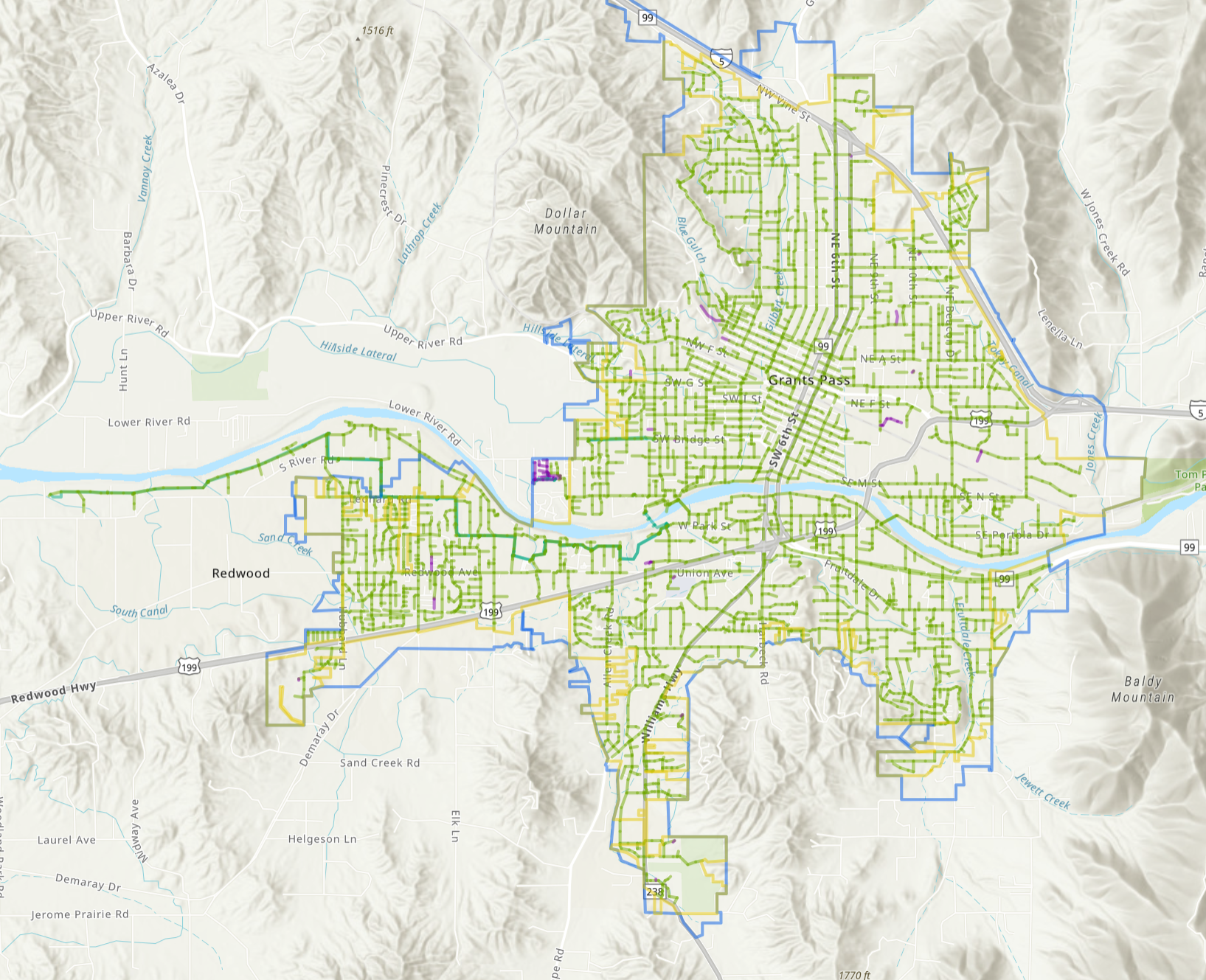
The wastewater network includes 277 km (172 miles) of gravity-fed sewer mains (see Figure 1) . After the closure of the Redwood Treatment Plant decades ago, the city installed 11 km (7 miles) of pressurized mains to pump the wastewater from lower elevations in the Redwood district to higher elevations that connect to the gravity-fed system. Last Thanksgiving a pump failure at the station forced a hurried repair while the well filled with sewage above the waists of the repair workers, so let's just say we like to keep the pressurized mains to a minimum.

The majority of existing service laterals are unrecorded, with only newer development including the assets, totalling 0.41 km (0.25 miles). Field crews note the location of service taps along the mains during CCTV inspections, and we use this as a secondary source to confirm taps identified in construction drawings, but often these CCTV reports are the only record of service taps that we have.

Figure 1. Grants Pass Wastewater Geometric Network

Initial Scope

The goal of our initial migration will be to achieve as direct a translation as possible of our existing network into the new Utility Network format. The downside of this approach is that we will leave many of the new features and functionality on the table: because our existing network is not z-aware, our import will have all elevations at zero, with key elevations recorded in attribute fields. Because we represent manholes as points in our existing network, we will not initially have any containments to represent the manhole structure.

No elevations, no containers... we cannot take advantage of any of the new features in the Utility Network! What sort of migration is this!?

The answer: incremental. Before we can take advantage of the neat things that Utility Networks can do, our assets have to follow the stricter rules that come with participating in the network. Type safety, within the context of geospatial science, means that we use the rules of the type system to make invalid states unrepresentable in the program. For our utility network, this means more stringent rules about what assets are allowed to connect, under what conditions. With these rules in place, we can ensure that certain properties hold over the network as a whole. The type-safe approach to network design makes possible a lot of exciting modeling applications that were not tractable using geometric networks on ArcMap.

The hard part of migrating our geometric network data is not adding elevations or containments, the challenge is to describe our existing data in a way that adheres to the stricter connectivity rules of the Utility Network model. Once we have raised our data quality to adhere to these standards, then we can iterate on our design with greater liberty. It is much easier to experiment with adding elevations or containments to an existing Utility Network, than to try to bolt all this stuff on during the import process. Again, we need to walk before we can run.

Project Setup

I have created a new ArcPro project called "wastewater_pilot_2026", to centralize files related to this migration.

The first step is to import a local copy of the wastewater assets into the project, and to do this I create an empty GDB called "wastewater_gn" within the project folder. This geodatabase will hold a defensive copy, allowing us to perform transformations on the source data without affecting our production use.

A Defensive Copy

We run an Enterprise stack, currently on version 11.5. Our wastewater geometric network is located on our Enterprise database, and uses Traditional versioning. The projection is NAD 1983 StatePlane Oregon South FIPS 3602 (Intl Feet). While it is possible to import the data into a Utility Network directly from the database, I recommend making a copy of the data in a local GDB, and importing from this local copy instead. I recommend this for a couple reasons: first, importing from a local copy can be faster and less error prone; and second, it can be helpful to perform transformations on the source data before import that you don't want to do to the source data itself. In my case, I want to project the data into a new projection, and remove attachments on layers where we no longer use this approach and the existing attachments are out of date.

After some time juggling four separate projections in use at the City when I arrived, eventually I consolidated all our published services into OCRS Grants Pass-Ashland NAD 1983 2011 TM (Meters). First off, we are a very small city to have a projection named after us, so it seems like a shame not to use it. Second, I developed a taste for the metric system while earning my PhD, and after measuring difficult things in this system, you don't want to go back. Third, I am absolutely sick of the English measurement system. What a God-awful antiquated throwback way to measure! We will be using meters and converting to miles and feet only for "legacy support", which currently includes everybody else at the City.

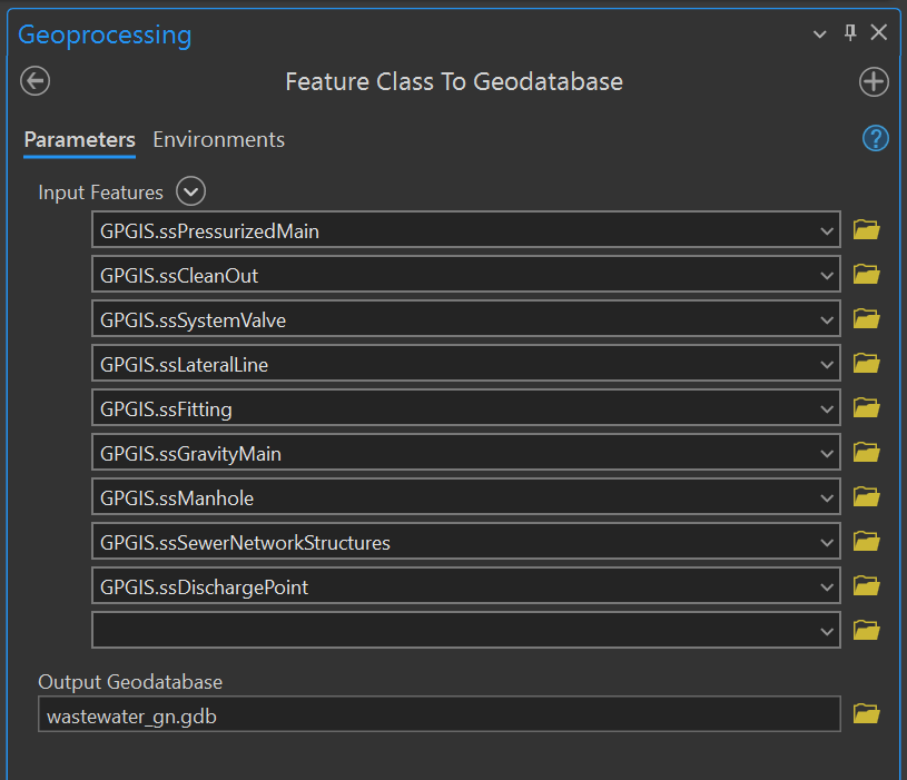
Let's examine the tool call we use to create the backup copy of our geometric network. In the parameter dialog for the Export Features tool, we have included all layers of the geometric network for wastewater with the exception of the net junctions layer, as this layer only contains bookkeeping for the geometric network, and will not be necessary to build the new Utility Network, (see Figure 2) .

Figure 2. Wastewater GN Import

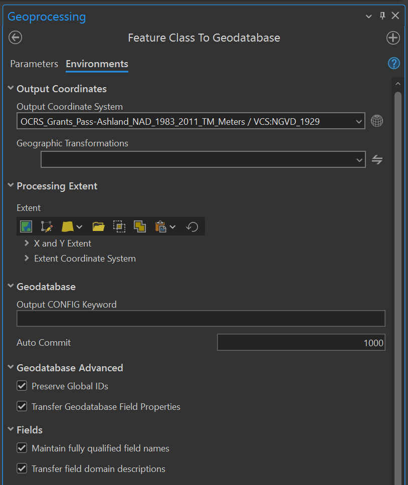
There are a few key boxes in the Environment tab checked here that are unchecked by default (see Figure 3) :

• First, I have elected to Preserve Global IDs. Assets in the wastewater geometric network have existing global IDs, and we want to retain these when we import our assets, so that we can cross-reference assets between the old and new datasets. Although we can join the old layer to the new using identifiers like the facility ID, global IDs are the idiomatic ESRI way to track our assets across the boundaries of a migration like this.
• Second, I have elected to Transfer Geodatabase Field Properties. We select this option so that the copy GDB will share the same Domains as data in the source. If you have short-coded domains, with integers as keys and text as descriptions, this will preserve the descriptions and import the Domain, otherwise you will just get raw integers with no context in your copy.
• Third, I have elected to Transfer field domain descriptions. Since we are importing Domains, let's import their descriptions as well.
• Finally, I have set the output coordinate system to OCRS Grants Pass-Ashland NAD 1983 2011 TM (Meters). Note that in the absence of a proper metric vertical datum, we are using NGVD 1929 in feet for elevation, which matches the format of all the elevation data in our attribute fields.

Figure 3. Import Environment

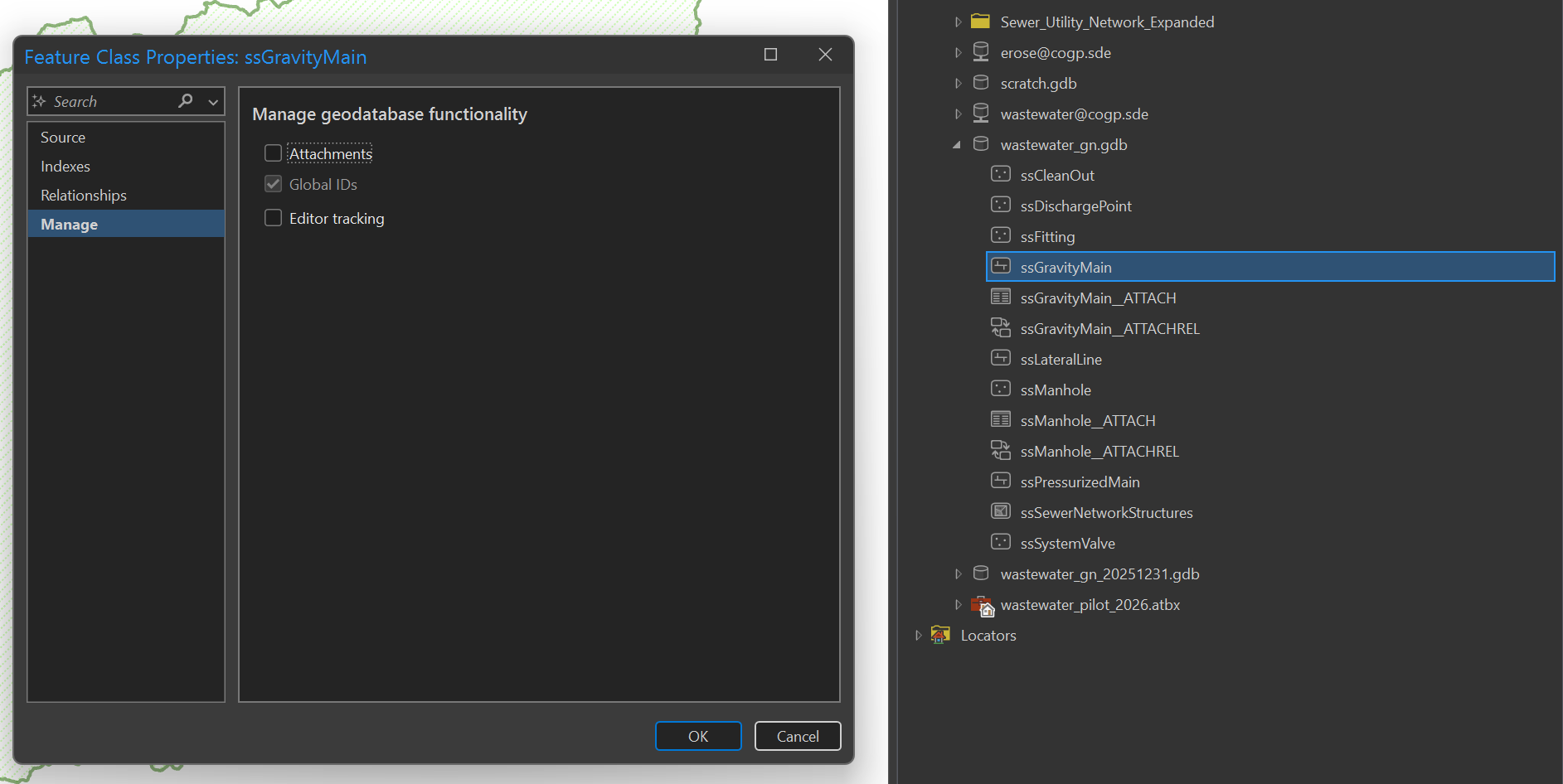
In the past, our field workers would attach pdfs of the manhole cards directly to the points in the manhole layer, and CCTV reports to the line assets in the mains layer. I am not a big fan of these attachments on our core utility layers; they create import and export issues, bandwidth issues, and generally these layers are a poor place to store giant image files. Instead, we centralize image storage and link to the storage location, so that our geospatial layers only have to include the link text in an attribute field, instead of hauling around a giant attachment.

In our defensive copy, I use the Manage tab in the Feature Class Properties pane to remove attachments from both the gravity mains and manholes layers, then press OK (see Figure 4) . Note that I am not advising you to strip images from your dataset, as this is not a mandatory step for importing into a utility network... I am just taking you through the blow-by-blow of how we are doing it in Grants Pass, with some minimum justification of why.

Figure 4. Removing Attachments

Download the Sewer Utility Network Foundation

From AGOL or your Enterprise portal, select the Solutions platform from the waffle menu of ESRI apps, enter "Sewer" into the search bar, and select the Sewer Utility Network Foundation solution. Hit the Deploy Now button, which will create a copy of the solution in your account. You can see "deployed" solutions in the My Solutions tab, which should now include the Sewer Utility Network Foundation package. In the item page for this solution, note the Solution Contents card lists three items:

• Combined Sewer Utility Network Essentials
• Sewer Utility Network Essentials
• Sewer Utility Network Expanded

The one-line description for the Expanded option says that it includes support for both combined and separate sewer systems. Our sewer system is separate from stormwater, but we have exceptions in gas stations, where we use sanitary sewer catch basins and route surface runoff into oil/water separators. Maybe the Network Essentials would be adequate for our needs, but I get greedy and want the Expanded options, just in case we need them, so I have copied the Expanded version into our working directory by downloading it from the "deployed" package on AGOL.

I move the contents from my Downloads folder into the project workspace. The contents look like this:

Sewer_Utility_Network_Expanded/
├── Data Model/
│ ├── SanitaryOnly_Configuration.gdb
│ └── SewerExpanded_AssetPackage.gdb
├── Sewer Utility Network Expanded.gdb
├── Styles/
├── Toolboxes/
├── Sewer Utility Newtwork Expanded.aprx
└── Sewer Utility Network Expanded.atbx

If you were to load the .aprx project file, it would show a bunch of demo data for Naperville, Illinois, designed to showcase features of the Utility Network for curious potential adopters. Most of this show is unnecessary for us; we have already committed to buying the cow and do not need to taste the milk. The only file we need is actually the Asset Package, stored as SewerExpanded_AssetPackage.gdb. However, there are a couple issues with our freshly-downloaded Asset Package. First, the spatial projection of the package is NAD 1983 StatePlane Illinois East FIPS 1201 (US Feet), which is reasonable to showcase the demo data in Naperville, but not ideal for the Pacific Northwest.

To resolve this issue, we will use the Change Asset Package Spatial Reference tool in the untools toolkit, a third-party Python library that we will need to download and install.

Download the untools package

The untools toolkit is a third-party Python package that does not come bundled with ArcPro. ArcPro allows us to download third-party Python packages and use them in our projects, but we have to go through a few extra steps to make that happen. We will follow the instructions from the docs here.

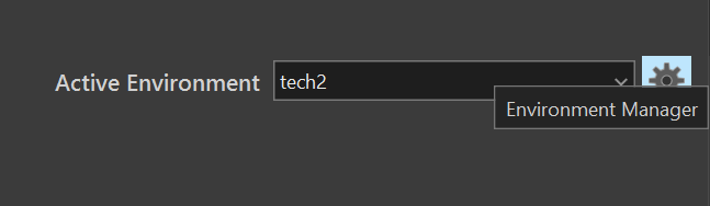
I favor using the GUI interface, selecting the Project tab from the menu bar, and then the Package Manager tab. At the top right, the Active Environment dropdown identifies the name of the current environment. Select the gear icon next to the dropdown to open the Environment Manager pane (see Figure 5) .

Figure 5. Open the Environment Manager

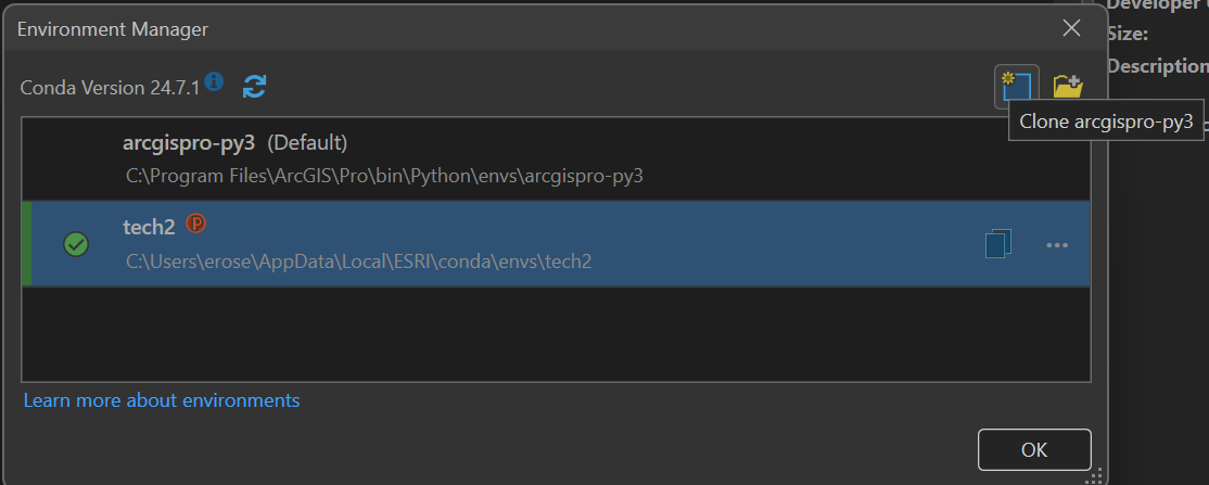
ArcPro does not allow us to add packages to the default environment. To customize our environment, we need to create a named copy that is safe to modify. To do this, we will use the Clone Environment button in the Environment Manager pane to create a copy using the name of our choice (see Figure 6) . In this case, I have already created a cloned environment named tech2. If you already have a custom environment, you can simply add untools to your cloned env, no need to make a new version then.

Figure 6. Clone the Environment

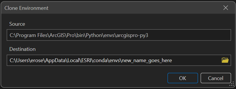
If you do need to create a new environment, the dialog for the clone operation will allow you to specify the target destination, which defaults to the hidden local AppData folder. The default location is generally fine, but you will need to specify a unique name for your clone (see Figure 7) .

Figure 7. Name and Location of Environment

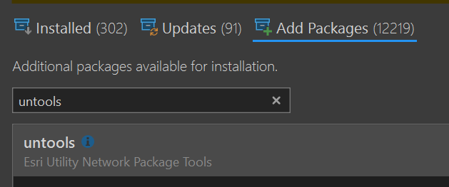
When you switch to a new environment, ArcPro will prompt you to restart. Do this, and then return to the Package Manager tab. Above the search bar, click on the Add Packages tab. In the search bar, type in "untools" and the package will appear as the sole option in the list of results (see Figure 8) .

Figure 8. Search for untools

To the right of the package list, details of the selected package will appear in the Package Details pane. At the top right of the pane, click on the Install button to add this package to your cloned environment (see Figure 9) . Agree to the Terms and Conditions and press OK.

Figure 9. Install untools

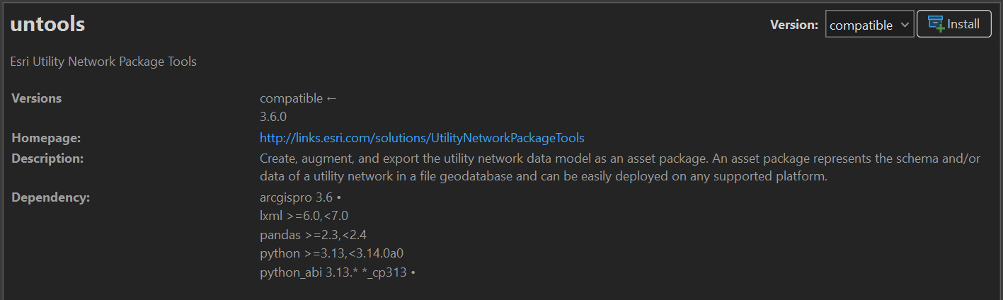
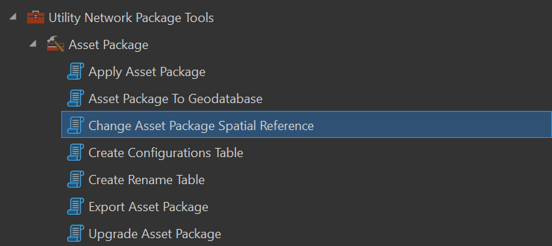
Once installation is complete, the Utility Network Package Tools toolbox will be available in the Geoprocessing Pane, including the Change Asset Package Spatial Reference tool (see Figure 10) . In addition, we will also be using the Asset Package to Geodatabase and Export Asset Package tools during the migration process.

Figure 10. Utility Network Package Tools

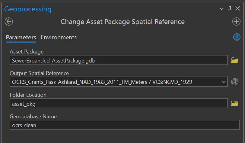
Change Asset Package Spatial Reference

When we examine the tool call for the Change Asset Package Spatial Reference tool, I have opted to place the output in a subfolder within our project called asset_pkg. I have set the spatial reference to match the projection of our source data, as we copied it to wastewater_gn. I have named the asset package "ocrs_clean", because we are using an OCRS projection, and because this is a "clean" version that we can copy and use for repeated loading attempts (see Figure 11) . Mistakes and failures during the import process can leave the asset package in a messy state, and it can be convenient to have a clean copy that is already configured for use, in this case with the correct spatial projection. As we get further into the import process, you will discover the process is iterative, and we will make other changes to the asset package as well. Having a clean copy of the fully-configured version can streamline the effort of making multiple import attempts.

Figure 11. Change Asset Package Spatial Reference

This tool creates a copy of the target asset package in the specified location, so after the tool run, our project directory will look like this:

wastewater_pilot_2026/
├── asset_pkg/
│   └── ocrs_clean.gdb
├── Sewer_Utility_Network_Expanded/
├── wastewater_gn.gdb
└── wastewater_pilot_2026.aprx

Set the Service Territory

The Service Territory is a polygon feature class of one or more features that spans the operational area of the network. The extent of the features in this layer defines the extent of the Utility Network, meaning inside this area you can add features to the network, and outside you cannot.

Why do we have to specify the extent of our service territory beforehand? According to Remi Myers, Product Manager for the ArcGIS Utility Network, on the ESRI Community Forum:

The reason behind the service area was to create the optimal indexing structures for the utility network. These structures include the index on the dirty feature class and the future spatial partitioning of the network index. So creating a service area that is bigger than needed will have a potential negative side effect in that the spatial index is not going to be optimal but it will still function.

The advantage of choosing a Service Territory that is "just right" is faster, more optimized lookups. Who doesn't want their maps to be fast? The disadvantage of choosing a service territory "too small" is that it may fail to accommodate future growth, requiring refactoring of the network down the line.

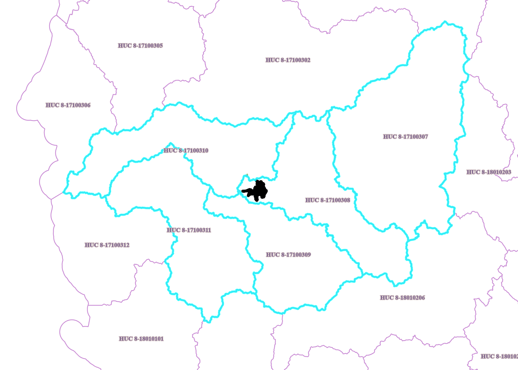
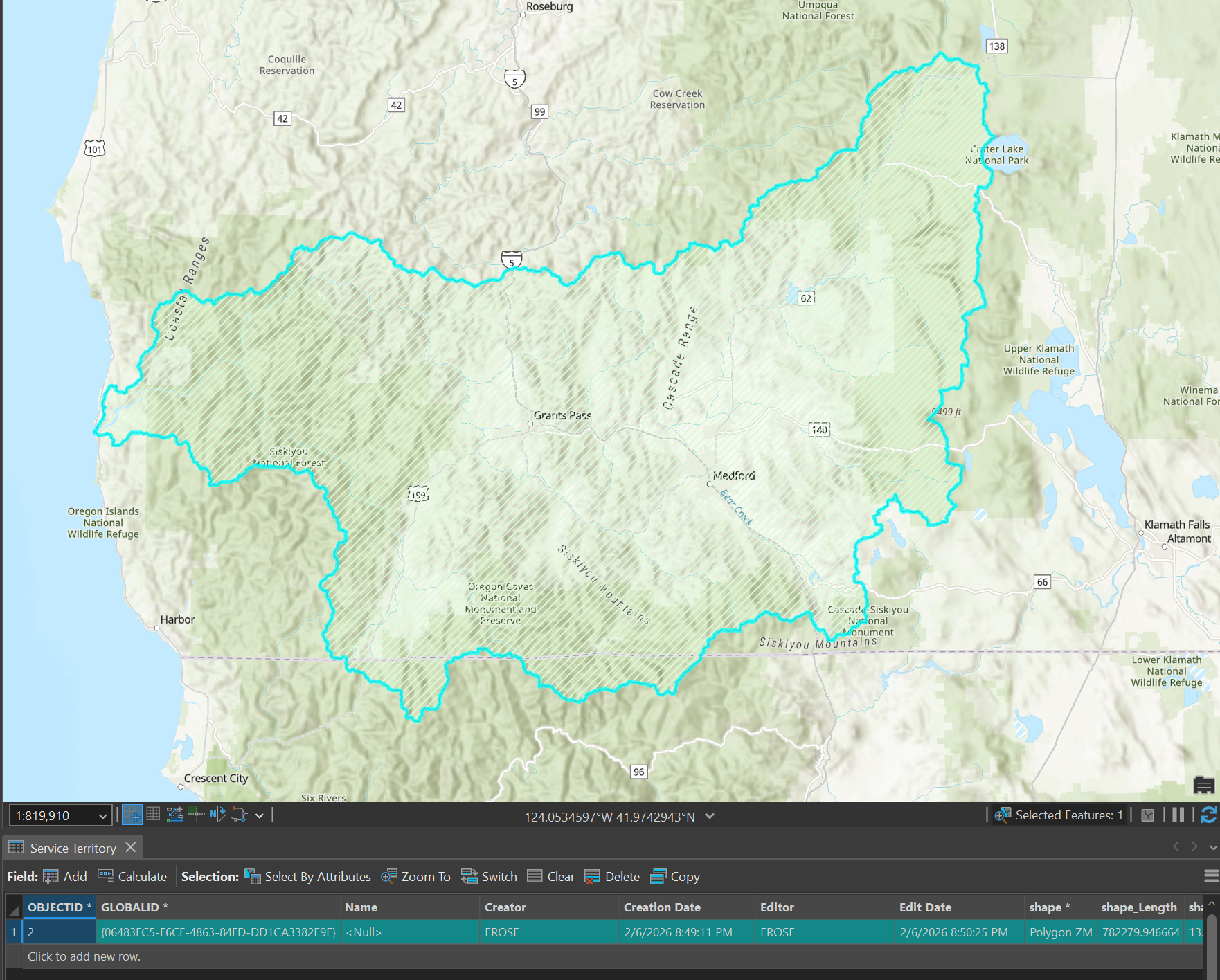
As an environmental scientist, I tend to reach for watershed boundaries to delineate regional areas, which provide boundary lines that make sense for the topography. We are going to characterize our service territory as as the greater watershed associated with the Grants Pass area. Using the 8-digit boundary codes from the NRCS Watershed Boundary Dataset, I have highlighted the surrounding watersheds, including a generous portion to the east that produces the majority of our drinking water (see Figure 12) . It begins in the easternmost portion at Crater Lake, visible in the map image as a large semi-circle in the drainage area, and terminates at the westernmost portion, where the Rogue River drains into the Pacific. This area should be small enough to keep acceptable performance characteristics, but large enough to satisfy even the most expansionist City Council.

Figure 12. Watershed Boundaries for the Grants Pass Area

First I export the highlighted polygons to the project GDB, then I use the Pairwise Dissolve tool to merge the separate boundaries into a single polygon. In the active Map, I add the Service Territory layer from ocrs_clean, which should still be empty. Using the Append tool, I add the newly-created polygon to the Service Territory layer (see Figure 13) . Because the dissolve operation stripped away the GlobalID field, I found that the polygon imported with an (invalid) GUID of all zeros. To fix this, I selected the field in the Attribute Table and hit the plus button to generate a new GUID.

Figure 13. Grants Pass Service Territory

All that being said, I could have just drawn a box around the assets in our existing dataset and called it a day. It would have been fine. You could even argue my version is worse, because it is larger than necessary. At least I find it aesthetically pleasing.

Conclusion

This concludes the setup process for our wastewater migration. I know -- we haven't done any actual migration yet! What we have done is installed the required tools, downloaded the necessary source materials, and created a focused project space. We have projected our destination asset package into our target spatial projection, created our service territory, and now we are ready to actually start importing. For our blog series, we will continue to break down the elephant migration process into digestible article-sized bites. In the next post, we will examine how to use the Data Loading tools to import our assets from the source data into the target schema. Stay tuned!