UN Wastewater Migration: Data Loading Intro

Erik Rose published on February 17, 2026

12 min, 2201 words

Categories: Tutorial

Introduction

When many of us started receiving deprecation warnings for geometric networks from ESRI years ago, we shook our heads ruefully. Who has time to migrate? Not now! If you are like me, you have kicked the can down the road year after year, and now 2026 is here. As of March 1st, geometric networks are no longer officially supported, and we haven't migrated yet. If you are in the same boat, do not worry. In this blog series, we will take you step by step through our UN migration at the City of Grants Pass. You will share our suffering, learn from our mistakes, and by the end I hope you will feel new confidence for tackling this migration in your municipality.

This is the second post in our UN Wastewater Migration series. In the first post, we cover project setup, including installation of the untools package and downloading the Utility Network Foundation. Today, we will introduce you to the Data Loading tools, and give you a brief tour of the DataReference sheet that you will use to orchestrate the import process.

Using the Data Loading Tools

For several years, the Data Loading tools have been fighting their way into legitimacy. Starting in ArcPro 3.2, the Data Loading tools now come bundled in the Data Management Toolbox. We will be using these tools to read assets from our geometric network and load them into the destination utility network, while preserving key attribute data, and mapping values from existing domains into our target schema.

The first tool we need is called Create Data Loading Workspace. This tool will create a subfolder within our project workspace, and populate this directory with a series of spreadsheets that describe the source and target schemas. Inside the asset_pkg subfolder of our project workspace, we have placed a copy of our target Asset Package called ocrs_clean. The import process will be iterative, and we will want the option to start over fresh with a properly configured asset package, so instead of working with the ocrs_clean package directly, we are going to make a working copy of the asset package that I will call working_ap.

No fancy ESRI tool needed here, I just copy, paste and rename in Windows File Explorer. When we select Target layers in the tool properties dialog, we will use layers in working_ap and keep ocrs_clean read-only. For each Source and Target pair identified in the tool parameter window, the tool will compare the schema in the source to the schema in the target. The challenge for us is to identify the correct destination layer in the Utility Network for each source in our wastewater geometric network (see Figure 1) .

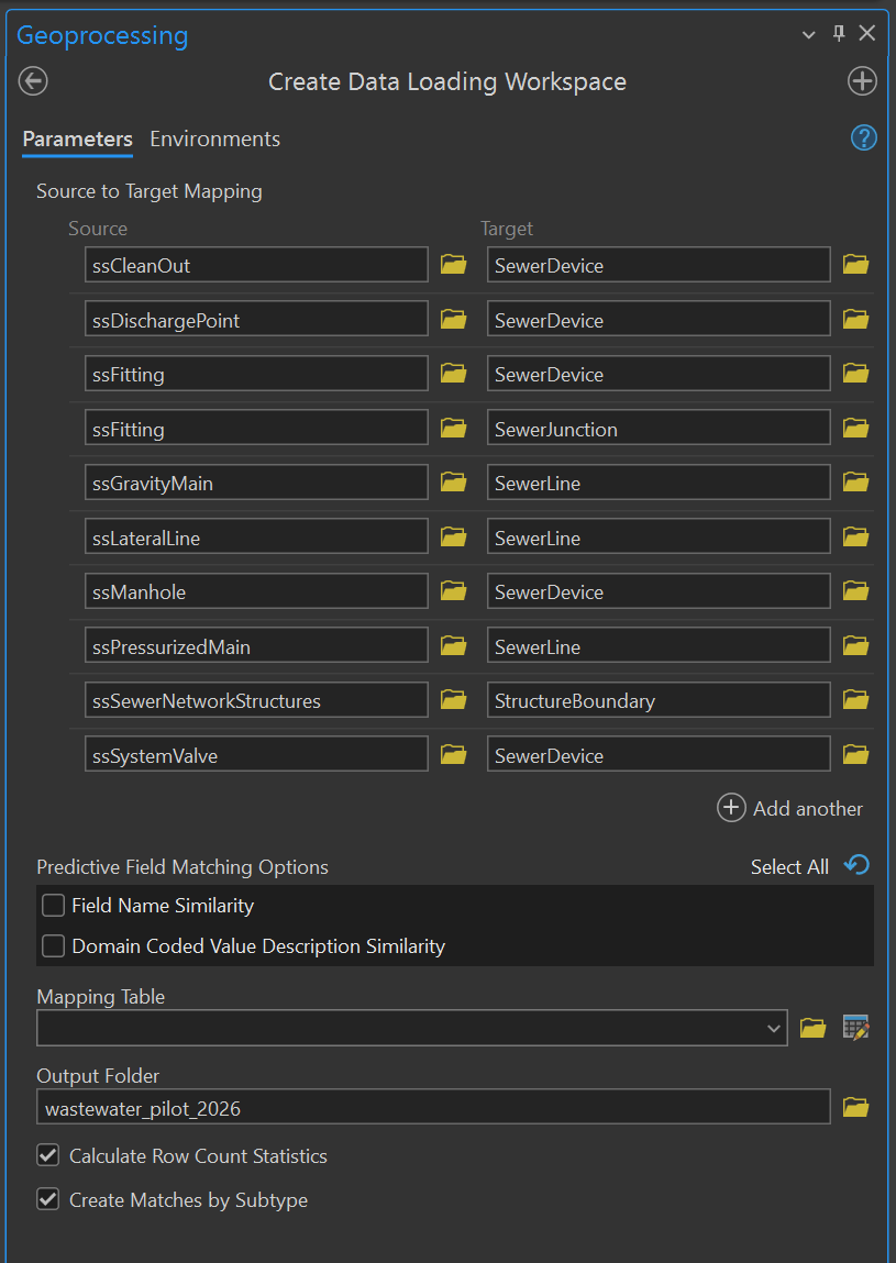
If I click on any of the Source or Target fields, it will show the full path, where our source data points to wastewater_gn, and our target data points to working_ap. For cleanouts, we map assets in wastewater_pilot_2026/wastewater_gn.gdb/ssCleanOut to the destination layer wastewater_pilot_2026/asset_pkg/working_ap.gdb/UtilityNetwork/SewerDevice.

Defining Source and Target Relations

There are a couple of interesting things we can note, just by scanning the layer names. First, the relationship between sources and targets can be many to one. Cleanouts, outlets, manholes and valves all map to the same target layer: SewerDevice. Utility Networks make heavy use of sub-typing to discriminate between different asset types within the same point, line or polygon layer. Consequently, Utility Networks have fewer data layers doing heavier lifting. Points that participate actively in the network are Devices, whereas structural elements are Junctions. Mains and lateral services both map to the same SewerLine type.

However, the relation can also be one to many. Note that we have ssFitting in there twice as a Source, first with SewerDevice as a target, and then SewerJunction. Generally speaking, we use our fittings layer to track pipe fittings, but not always. Since the humble fitting is so innocuous, my predecessors used it as a catch-all for things that otherwise had no home layer. Over time, the Domain assigned to our fittings grew from a reasonable list of pipe fitting types, to include types like "Service to Address Point", "Stand Pipe" and "Blow Off Port". We have a situation where some of the points in our fittings layer need to map to one target, and some to another, and the Data Loading tools will allow us to fine tune this splitting process.

The Data Loading Workspace

I am happy to extend this domain abuse pattern to facilitate the migration process, in ways I will explain below. First, let's take a look at what happens after you run the Create Data Loading Workspace tool. Inside your project folder, you will find a new subfolder called DataLoadingWorkspace, with the following file layout:

wastewater_pilot_2026/
├── asset_pkg/
├── DataLoadingWorkspace/
│   ├── Data Mapping/
│   │   ├── GlobalLookup/
│   │   ├── Points/
│   │   ├── Polygons/
│   │   ├── Polylines/
│   ├── Domains/
│   │   ├── wastewater_gn.gdb.xlsx
│   │   └── working_ap.gdb.xlsx
│   ├── Scripts
│   └── DataReference.xlsx
├── Sewer_Utility_Network_Expanded/
├── wastewater_gn.gdb
└── wastewater_pilot_2026.aprx

With the exception of the Scripts folder, it is Excel sheets all the way down. These sheets describe the source and target schemas, and provide us with a (somewhat crude) framework for defining relations between fields in the source and target layers. We will explore the Data Mapping and Scripts folders in greater detail soon. For now, focus in on DataReference.xlsx, as this is the entry point for the loading configuration process. DataReference contains links to the Excel sheets within the Data Mapping and Domains folders, so you will have very little need to open and navigate these folders directly, rather you will open DataReference and navigate through the stack using doc links.

DataReference Tour

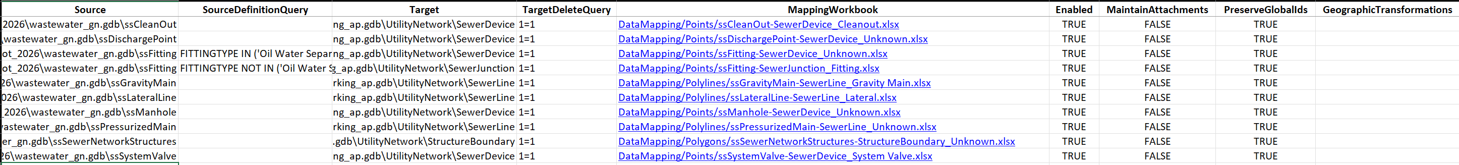
Let's take a quick tour of the DataReference Excel sheet (see Figure 2) . When you open the document, you will see nine columns:

Source
SourceDefinitionQuery
Target
TargetDeleteQuery
MappingWorkbook
Enabled
MaintainAttachments
PreserveGlobalIds
GeographicTransormations

Source & Target

The Source column lists the fully-qualified path to each layer in the geometric network, and the Target column shows the path to the destination layer in the Utility Network. The sheet will have one row for each Source & Target pair specified in the Create Data Loading Workspace tool. In our case, we have 10 rows for the following transformations:

ssCleanOut -> SewerDevice
ssDischargePoint -> SewerDevice
ssFitting -> SewerDevice
ssFitting -> SewerJunction
ssGravityMain -> SewerLine
ssLateralLine -> SewerLine
ssManhole -> SewerDevice
ssPressurizedMain -> SewerLine
ssSewerNetworkStructures -> StructureBoundary
ssSystemValve -> SewerDevice

Definition Queries for Sources

The SourceDefinitionQuery column contains SQL statements that restrict the records in the source layer to a subset of the total, the same way a Definition Query works on layers in a project map. When the relation between the source and target layers is one to many, definition queries on the source layer are how we partition the data so that only data that meets the query migrates to the destination layer.

For our dataset, we map the fittings layer to both SewerDevice and SewerJunction types in the destination network. In the SourceDefinitionQuery column, we include the following SQL statements:

ssFitting -> SewerDevice: "FITTINGTYPE IN ('Oil Water Separator', 'GreaseTrap', 'Service To AddressPoint', 'SS Catchbasin', 'Pump')"
ssFitting -> SewerJunction: "FITTINGTYPE NOT IN ('Oil Water Separator', 'GreaseTrap', 'Service To AddressPoint', 'SS Catchbasin', 'Pump')"

Note that the only only difference between the two statements is the word "NOT", defining everything inside the set as devices, and everything outside as junctions. Inside the statement, we are selecting domain values that will map to device types in the new Utility Network. This is how we avoid importing the same assets twice, as devices and junctions.

Target Delete Query

The TargetDeleteQuery column takes an SQL statement that selectively deletes data from the target dataset before loading. We almost exclusively use the expression "1=1" to delete all data from the target layer before the next attempt to load. Note that you can use SQL-fu to delete subsets of your data, such as:

Status = 'Inactive' to delete only records where the Status field is Inactive.
Date < '2023-01-01' to delete records older than a certain date.
Category IN ('A', 'B', 'C') to delete records belonging to specific categories.

However, the primary use case is to delete the previous loading attempt. During the initial import process, we will be fiddling with the import instructions, making small changes, and loading again, and will almost certainly want the previously-loaded data removed. Therefore, I will use the value of "1=1" for each row.

Mapping Workbook

The MappingWorkbook column contains a link into the DataMapping folder of the loading workspace. For each row specifying a Source and Target, the Data Loading tools create a unique spreadsheet in the Points, Polylines or Polygons folders, using a "{source}-{target}_{subtype}.xlsx" naming convention. The cells do not just list the path to the folder, they function as jump links: clicking on them will open the selected sheet. We will be using these links to navigate the data loading workspace. You will not need to edit or alter these fields, just click on them occasionally.

Import Enabled

The Enabled column indicates whether the Data Loading tools will process the row. This column is a blessing when migrating large datasets, because it allows us to skip some rows entirely while we target and refine imports on another layer. During the initial import process, we will leave Enabled set to TRUE only for the active layer we are working on, and FALSE for all other rows. We will not set all rows to TRUE until we are ready to perform the final import.

Maintain Attachments

The MaintainAttachments column indicates whether the Data Loading tools will include attachments when it imports data from the source layer. You may recall in Part 1 that we deleted the attachments from our source data, because we did not need them in the new network. Deleting the attachments entirely results in a slight performance boost during loads, since the size of the source dataset is smaller. We already deleted all our attachments, so the value of the rows in this column will not impact our import, but generally speaking you can ignore attachments during import using FALSE and honor them using TRUE.

Preserve Global IDs

The PreserveGlobalIds column indicates whether the Data Loading tools will honor and copy over the Global IDs present on the source layer. Selecting TRUE will preserve the IDs, and selecting FALSE will ignore them. Since we rely on Global IDs to establish a link between assets in the source and target layers, we want to preserve them. In fact, when we were making a local copy of our source data in Part 1, we specifically had to check a box to preserve Global IDs from the Enterprise GDB on our local copy. Selecting TRUE to preserve Global IDs is the next step in transferring those IDs into our destination layer. We set PreserveGlobalIds to TRUE for all import layers, so that the IDs of new assets in the Utility Network will match their corresponding asset in the old geometric network.

Geographic Transformations

The GeographicTransformations column allows you to re-project the source data into a target spatial reference by specifying the transformation string as the row value, for e.g. "MGI to WSG84". If you remember from Part 1, we already transformed our source data into the target spatial reference when we copied our Enterprise data onto the local GDB. Why did I bother, if we can just specify the transformation here? If I had confidence we were going to succeed on the first try, then I would encourage you to leave the transformation in the worksheet, as we would only the pay the cost once. But since we will be loading iteratively, trying an idea, making adjustments, and trying again, we will have to pay the cost for this transformation every time. Therefore, it is faster to perform the conversion once on the source GDB, leaving less work for the Data Loading tools to do on each run.

Conclusion

This concludes the tour of the DataReference sheet, and our brief introduction to the Data Loading Tools. You have learned how to run the Create Data Loading Workspace tool, discovered the layout of the loading workspace and explored how to read the DataReference sheet. You may be wondering when we will actually start importing data... In the next article, we will use the DataReference sheet to configure import of cleanout assets from our source data into the target network!

If you have questions, advice or war stories of your own, I hope to hear from you. Drop me a line at erose@grantspassoregon.gov. And stay tuned!